VLOOKUP, HLOOKUP, MATCH, INDEX and CHOOSE Function in Excel
Lookup and References
Lookup and Referencing is a very important feature of MS Excel. This feature allows users to learn all about MS Excels lookup & reference functions such as the VLOOKUP, HLOOKUP, MATCH, INDEX and CHOOSE function.
These functions help a user to work with data arrays in MS Excel, and are quite useful for cross referencing between different datasets. These functions perform tasks like getting information from a range, returning the address of a given value, or looking up for specific values.
VLOOKUP
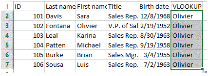
VLOOKUP (Vertical lookup) function searches for a defined value in the first column of the range, and then returns the values from the specified adjacent cell. In the example below, you will observe that the VLOOKUP formula contains 4 sections. The first section refers to the value to be searched for (i.e. 102), the second section holds the absolute range from where the whole VLOOKUP function will perform (i.e $A$2:$E$7), now the third section holds the information regarding the desired column whose respective value is to be displayed (i.e. 3 (column C)), and finally the final section that defines if the search would be fully matched or not. This is an optional value to be set.
1. Now, insert the VLOOKUP function shown below.
2. Drag the VLOOKUP function in cell F2 down to cell F7.
Note: when we drag the VLOOKUP function down, the absolute reference ($A$2:$E$7) stays the same alongwith the absolute value 102 also remains the same. However, if we had applied a relative reference, it would have changed to A4, A5, etc.
HLOOKUP
HLOOKUP functions in a similar way like VLOOKUP however, unlike VLOOKUP, if functions horizontally rather vertically. It operates on row instead of a column.
In the above example, you will observe that all the sections are same, however, the orientation has been switched from column to row.
Match
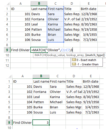
Match functions is use to detect the occurrence of a specified value within a given range and it returns the occurrence location in number format. In the example given below, you will observe that the function is required to detect the occurrence of “Olivier” in the provided range from C1:C7.
The function has found the desired value on 3 cell in the range (i.e. C3)
Index
The INDEX function returns a residing value in either a two-dimensional or a one-dimensional range.
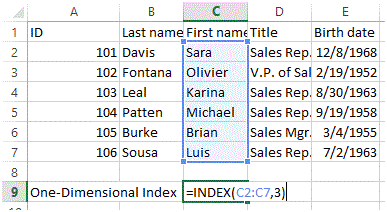
In the example above, you will observe that the Index function has been applied to range C2:C7 and the row index is 3. So the function will return the value of 3rd row in the given range (i.e. Karina). This is the example of one-dimensional
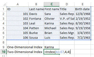
In the example above, you will observe that the Index function has been applied to range A1:A7 and the row index is 4. However, there is an additional allocation of column index which is also 4. So the function will return the value of 4th column on 4th row in the given range (i.e. Sales Rep.). This is the example of two-dimensional.
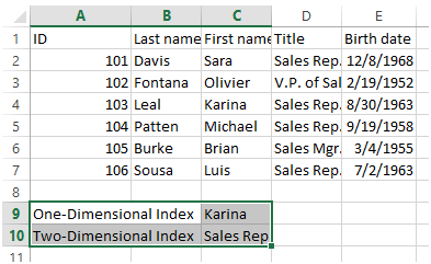
The above figure shows the return values of both examples.
CHOOSE
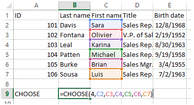
The CHOOSE function returns the value based on the index number from a given set of values. The function gets to the position index in values set and return the value residing on that particular position.
In the above example, the position index given is 4 hence, the function will return the forth value in the value set which is cell C5 (i.e. Michael).


