Formulas and Functions in MS Excel
Formulas and Functions in MS Excel
MS Excel is quite renowned for its excellent support for complex calculations and built-in formulas and functions. It also provides the flexibility to use these formulas and functions in an entirely convenient manner. As long as you have the understanding and knowledge of what you want to implement, MS Excel provides you with the platform to implement it.
What is a formula?
A formula is an arithmetic expression that calculates the values provided in the given range. It performs the intended operation (i.e. +, -, *, /, etc.) on the provided values and generates the desired output.
What is a function?
A function is a procedure defined in MS Excel to execute the formulas with more ease and efficiency. An example of a function is SUM(). Normally, if you sum the values of two cells (A1 and B1), you would write a formula like A1 + B1. Now, the same can be obtained using the SUM function. The syntax would be SUM(A1:B1).
The advantage of using the function is when you have to calculate more number of values like for instance if you are required to sum the values of Cell A1 to Z1, it will take you some time to generate the formula however, in SUM function, you will just type SUM(A1:Z1). This will select the whole range and will apply the SUM function to produce the desired result.
The above explanation is provided to give you the general understanding that how effectively MS Excel facilitates the users with meeting their requirements.
Procedure for entering formulas
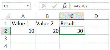
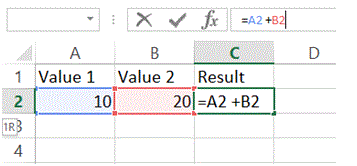
Entering formula is quite simple, as illustrated in fig.bel, Value 1 and Value 2 are assigned to Cell A2 and B2. Now, the result was required in Cell C2.
Therefore, the formula is written in C2 as “= A2 + B2, where A2 and B2 are cells containing values and “+” is the operation to be performed. Now the most important element of any formula or function is the “=” sign. This sign is the instruction point for MS Excel that anything written afterwards, will be a formula or a function and will be executed.
Now, let’s see some general step by step examples of entering formulas.
Example 1: Applying a formula
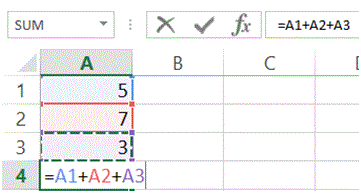
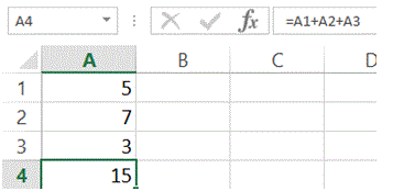
In this example, you will observe a “+” formula implementation on Cell A1 to Cell A3. The result will be shown in Cell A4
1. Enter 3 values in Cell A1 to A3
2. Select Cell A4, where the result of formula will be shown
3. Type “=” and click on Cell A1. You will observe a scrolling dashes against the cell. This refers that the cell has been marked.
4. Type “+” and click on Cell A2.
5. Again, type “+” and click on Cell A3.
6. Press “Enter” key.
7. Output of the formula will be displayed in Cell A4
Example 2: Editing a formula
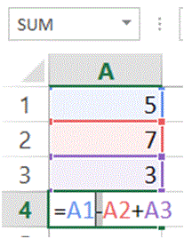
In this example, you will observe a change in the formula applied in Example 1, in which, “+” operation was performed. Now, in current example, the “+” operation will be changed with “-“ formula. There are two methods in which you can make the changes in the formula.
Method 1: Editing formula in output cell.
1. Double Click on the Cell A4. This will put the cell in edit mode
2. Change the “+” symbol with “-“ symbol
3. Press Enter key
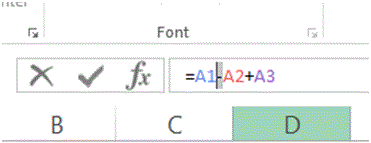
Method 2: Editing formula in Formula Bar
1. Select Cell A4
2. In formula bar, change the “+” symbol with “-“ symbol.
3. Press Enter key
Example 3: Copy/Paste a formula
Just like values in cells, MS Excel supports copy and pasting of formula as well. The operation is performed just like any other copy and pasting operation.
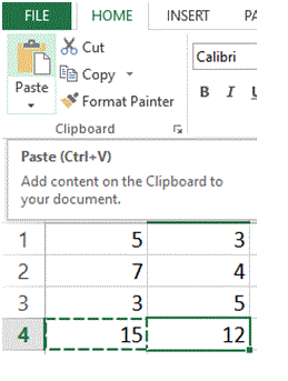
In this example, you will observe that, there are 3 values entered in Cell B1 to B3 but instead of typing the formula (as did in Example 1), a Copy function is applied on Cell A4 and Paste function is applied on B4.
1. Enter any numeric values in Cell B1 to B3
2. Select Cell A4
3. Click on “Copy” from Clipboard tab or Press “Ctrl + C”
4. Select Cell B4
5. Click on “Paste” from Clipboard tab or Press “Ctrl + V”
Applying a function in MS Excel
Applying function in MS Excel is as simple as applying a formula. You don’t need to do any complex tasks.
In the following example, you will observe the step by step implementation of SUM function on Cell A1 to J1 and the output result will be displayed on Cell K1.
Example 1 Application of SUM function.
1. Put numeric values in Cell A1 to J1
2. Select Cell K1
3. Type =SUM(A1:J1)
4. Press Enter key and the result will be shown in Cell K1
Example 2: Application of AVERAGE function
In this example you will be observing the application of AVERAGE function on the data from Example 1. The AVERAGE function will be implemented on Cell L1. This formula will be covering the values from Cell A1 to J1.
1. Select Cell L1
2. Type =AVERAGE(A1:J1)
3. Press Enter key and the result will be output on Cell L1
More Related Articles For You
- Important Terminologies in Microsoft Excel
- Working with Rows, Columns and Cells in Excel
- Working with Ranges in MS Excel
- Ribbon in MS Excel
- Workbook in MS Excel
- Formatting Cells in MS Excel
- Templates in MS Excel
- Data Validation in MS Excel
- Excel Keyboard Shortcuts
- Protecting a Workbook in MS Excel with Password
- Print Gridlines in an Excel Worksheet
- How to Share MS Excel Data
- Count and Sum Function in Excel
- Logical Functions in Excel
- Date and Time Function in Excel
- Worksheet in Excel
- Find and Select in Excel
- Cell References in Excel

