Count and Sum Function in Excel
Count and Sum Function in Excel
Count
The count function is MS Excel is very important. This function allows you to count the number of cells. The function has multiple variants that allow conditional counting. This tutorial will discuss these variants.
Count
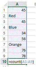
The count function is the basic function used for counting cells having numerical values. It doesn’t count cells with non-numeric data.
The syntax for Count function is =Count(“Cell Range”)
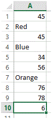
In the above figure, the total count is 6 which means, the formula has only counted cells with numeric values.
CountA
The CountA function is the basic function used for counting cells having all values. It doesn’t count blank cells data.
The syntax for CountA function is =CountA(“Cell Range”)
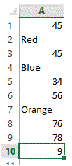
In the above figure, the total count is 9 which means, the formula has counted all cells with values. Please note that this function doesn’t count blank cells.
CountBlank
The CountBlank function is the basic function used for counting cells that are blank. It doesn’t count cells with values.
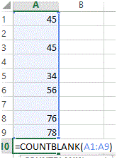
The syntax for CountBlank function is =CountBlank(“Cell Range”)
In the above figure, the total count is 3 which means, the formula has only counted cells that are blank.
Countif
Countif function is a conditional count function. It counts values in a given range on the basis of given criteria.
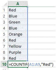
The syntax for Countif function is =Countif(“Cell Range”, “Criteria”). In the above figure, Range is defined from A1 to A9, whereas Criteria is set to Red. So now the formula will look for the word Red in the given range and will count its occurrence within the given cell.
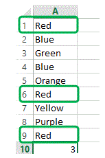
In the above figure, the total count is 3 which means, the word Red has occurred 3 times in the given range.
CountIfs
Countifs function is a conditional count function. It counts values in given ranges on the basis of given criteria. This function support multiple criteria for multiple range and the AND operation is performed between these criterias.
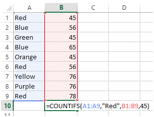
The syntax for Countifs function is =Countifs(“Cell Range 1”, “Criteria 1”, “Cell Range 2”, “Criteria 2”, ….). In the above figure, Range 1 is defined from A1 to A9, whereas Criteria 1 is set to Red similarly, Range 2 is defined from B1 to B9, whereas Criteria 2 is set to 45. So now the formula will look for the word Red in Range 1 along with having 45 as value in the adjacent cell in Range 2.
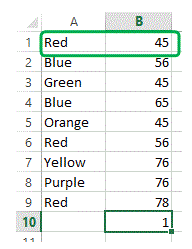
In the above figure, the total count is 1 which means, the word Red has occurred only 1 time when its adjacent cell in Column B had a value = 45.
SUM
The sum function is MS Excel is very important. This function allows you to sum the values of cells. The function has multiple variants that allow conditional sum. This tutorial will discuss these variants.
SUM
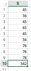
The SUM function is the basic function used for adding cells having numerical values.
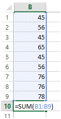
The syntax for SUM function is =SUM(“Cell Range”)
SUMIF
SUMIF function is a conditional sum function. It add values in a given range on the basis of given criteria.
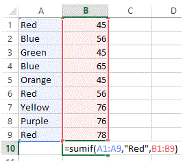
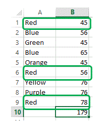
The syntax for SUMIF function is =SUMIF(“Range”, “Criteria”, “Sum Range”). In the above figure, Range is defined from A1 to A9, whereas Criteria is set to Red and the Sum range is set to B1 to B9. So now the formula will look for the word Red in the given range and will sum the adjacent cells in Column B.
In the above figure, the total sum is 179 which means, the word Red has occurred 3 times in the given range and the sum of its adjacent cells is 179.
SUMIFS
SUMIFS function is a conditional SUM function. It adds values in given ranges on the basis of given criteria. This function support multiple criteria for multiple range and the AND operation is performed between these criteria’s.
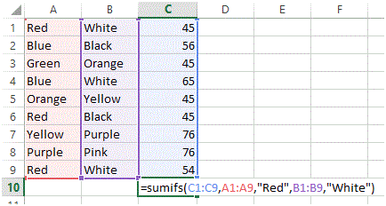
The syntax for sumifs function is =Sumifs(“SUM Range”, “Range 1”, “Criteria 1”, “Cell Range 2”, “Criteria 2”, ….). In the above figure, Range 1 is defined from A1 to A9, whereas Criteria 1 is set to “Red similarly, Range 2 is defined from B1 to B9 and Criteria 2 is set as White and finally the SUM Range is set to C1 to C9. So now the formula will look for the word Red in Range 1 along with having White in Range 2 and will perform sum function on cells where both criteria have been met.
In the above figure, the total sum is 99 which means, the word Red and word White has combine occurrence on2 points.
More Related Articles For You
- Important Terminologies in Microsoft Excel
- Working with Rows, Columns and Cells in Excel
- Working with Ranges in MS Excel
- Formulas and Functions in MS Excel
- Ribbon in MS Excel
- Workbook in MS Excel
- Formatting Cells in MS Excel
- Templates in MS Excel
- Data Validation in MS Excel
- Excel Keyboard Shortcuts
- Protecting a Workbook in MS Excel with Password
- Print Gridlines in an Excel Worksheet
- How to Share MS Excel Data
- Logical Functions in Excel
- Date and Time Function in Excel
- Worksheet in Excel
- Find and Select in Excel
- Cell References in Excel

